How Cassandra Streaming, Performance, Node Density, and Cost Are All Related

• Wed, Mar 5, 2025
• 15-minute read

This is the first post of several I have planned on optimizing Apache Cassandra for maximum cost efficiency. I’ve spent over a decade working with Cassandra and have spent tens of thousands of hours data modeling, fixing issues, writing tools for it, and analyzing it’s performance. I’ve always been fascinated by database performance tuning, even before Cassandra.

A decade ago I filed one of my first issues with the project, where I laid out my target goal of 20TB of data per node. This wasn’t possible for most workloads at the time, but I’ve kept this target in my sights.

I recently gave a talk called The Road to 20TB Per Node at an Apache Conference, where I laid out the improvements in the database that have impacted the amount of data a single node can hold, as well as laid out some optimizations that we can do to reach this goal.

At a high level, these are the leading factors that impact node density:

• Streaming Throughput
• Compaction Throughput and Strategies
• Various Aspects of Repair
• Query Throughput
• Garbage Collection and Memory Management
• Efficient Disk Access
• Compression Performance and Ratio
• Linearly Scaling Subsystems with CPU Core Count and Memory

In this series of posts, I’ll be examining how the above aspects of Cassandra architecture, starting with streaming operations, contribute to node density, directly impacting your operational costs. By understanding the considerations, and implementing the optimizations in this post, you can significantly increase the amount of data each node can efficiently handle. This will reduce the total number of nodes required for your cluster, decrease your operational overhead, and improve resource utilization, which will ultimately massively slash the cost of running your cluster.

Note: To fully leverage these optimizations, you should be running Cassandra 5.0 or later, which introduces significant performance improvements and multiple features specifically designed for higher node density. Many of the techniques we’ll discuss are most effective on this latest version, though I’ll note where certain optimizations apply to earlier releases as well.

In cloud environments, if you’re using disaggregated storage, increasing volume size is incredibly simple. For example, Amazon’s EBS allow you to increase volume size as an online operation without downtime. Storage is less expensive than adding both storage and additional servers. If you can pay for just disks, you can save a lot on your cloud bill.

Cost Impact: A Practical Example

Before digging into the details of streaming, let’s examine a real-world scenario using current AWS pricing (as of March 2025) to demonstrate the financial impact of increasing node density vs. horizontal scaling. For this post I’m using at EBS volumes, since it provides us a straightforward way of examining the cost difference. We can scale the volume size independently of the instance type. Changing instance types is also an option if you’re not using persistent disks, but we’ll keep things simple for this post.

This example assumes your bottleneck is not the bandwidth or IOPS of your disk. In future posts will examine some disk optimizations that can be done to improve disk efficiency. If you’d like to read a little about that now, I contributed a post to the AWS blog about optimizing EBS performance.

Scenario: Let’s say you want to double the amount of data you can store in your cluster. This is our cluster today. I’ve rounded the numbers off to keep things simple:

• 3-node cluster using m8g.4xlarge instances.
• Each node has 5TB EBS volume with 16K IOPS
• Disks cost approximately $500/month per volume
• Total cost of instances plus disk is $3,000 per month.

We have two ways to handle the additional storage:

Option 1: Horizontal Scaling by Adding Nodes

• To double capacity: Add 3 more m8g.4xlarge instances with 5TB disks
• Additional monthly cost: $3000 ($500 × 3 for instances + $500 × 3 for storage)
• Total Cost: Doubled, now $6,000

Option 2: Vertical Scaling by Increasing Node Density

• Same 3-node cluster with m8g.4xlarge instances
• Expand each 5TB EBS volume to 10TB (remaining at 16K IOPS)
• Additional cost per volume: $400/month
• Total additional monthly cost: $1200, 40% additional cost

Savings

Instead of our monthly cost doubling from $3,000 to $6,000, we only increase to $4200. This is a significant improvement, especially as your environment grows.

This difference doesn’t even account for the additional operational benefits of managing fewer nodes.

Efficient Streaming Makes the Option to Increase Node Density More Viable.

Let’s dig into the topic of this post, streaming.

Every time you add a node to the cluster, data needs to be sent from the live nodes to the new nodes. The process of adding a new node to the cluster is called “bootstrapping”, and the process for sending data to the node is called “streaming”.

Efficient streaming plays a crucial role not only in how fast we can scale, but also in maintaining high availability and minimizing the risk of outages when nodes fail.

Streaming in Cassandra occurs in these scenarios:

• When adding nodes (bootstrapping or rebuilding)
• When removing nodes (decommissioning)
• When replacing failed nodes, with replace_address_first_boot
• When running scheduled repair

In each case, the speed and efficiency of data transfer directly impacts your cluster’s stability and operational costs.

Expanding and Contracting

When we can add and remove nodes to (and from) the cluster quickly, we can handle dynamic workloads more effectively. It’s fairly common for ecommerce sites to scale clusters up around the holidays to handle additional traffic. If we need to double a cluster from 24 to 48 nodes, we want it to happen as quickly as possible. Scaling quickly means we can add nodes with less lead time, which has a huge impact on the cost of running your cluster.

Node Replacements

When replacing nodes via replace_address_first_boot, you want to minimize the window of vulnerability. While this is happening, the system is operating with reduced redundancy, since the incoming node hasn’t yet received a complete copy of its data. When looking at replacing nodes, consider these factors:

Vulnerability Window

• Longer streaming times mean extended periods where data isn’t fully replicated
• The cluster is operating with fewer copies of you’ve specified in your replication configuration
• If you’re using LOCAL_QUORUM with RF=3, another node failing can result in some data being unavailable
• Incremental repair is unavailable on ranges affected by the missing node
• Many other automations cannot be run during this window
• Depending on some circumstances, some data can become inconsistent

Performance Impact

• Streaming operations consume network bandwidth and system resources
• A failed node can’t respond to queries, meaning the remaining nodes need to service additional requests
• Other operational tasks may experience increased latency
• Resource contention can slow down regular client operations
• The remaining nodes are storing hints. In older versions of Cassandra this could introduce performance issues.

In all cases, the objective is to minimize this window, ensuring nodes become fully operational as quickly as possible while maintaining system stability. This approach strengthens cluster resilience and reduces the likelihood of cascading failures during node replacement or scaling operations.

While faster streaming contributes to cost savings through higher node density and efficient resource utilization, it is equally vital for minimizing the risks associated with node failures and ensuring uninterrupted cluster operations. By understanding and following the guidelines in this post, your clusters can achieve both improved scalability and reliability, while also minimizing cost.

Understanding Data Streaming Methods

With that out of the way, lets look at the three code paths streaming can follow, and I’ll show you how you can best take advantage of the fastest ones. Let’s take a look at each of them, starting with the best performing.

Zero Copy Streaming (ZCS)

ZCS appeared in Cassandra 4 (see Hardware-bound Zero Copy Streaming in Apache Cassandra 4.0) and is the most optimized form of streaming in the database. It makes use of a Linux system call, sendfile(), which is is an optimization for transmitting files over a network without needing to read the data into userspace, hence “zero copy”.

In Cassandra, we use this to stream entire SSTables directly from the filesystem to the network without intermediate buffering in the JVM heap. The code is found in SSTableZeroCopyWriter

To enable this feature, ensure the following is set in cassandra.yaml (it’s on by default):

stream_entire_sstables: true

How fast is fast? You’re basically limited by your disk and network throughput on the sending side.

Note: On the receiving side, your new nodes will still need to perform compaction on the data.

By now you might be wondering, if this is so awesome, why isn’t it used all the time? Well, there’s two caveats:

• ZCS can only be utilized when the entire SSTable will be owned by the destination node. There are a couple factors that affect this, which we’ll get into in the optimizations section.
• ZCS can’t be used (yet) if you’re using internode encryption

For partial transfers, Cassandra must fall back to the slower streaming path.

Encrypted Entire SSTable Streaming

Like Zero Copy Streaming, Encrypted Entire SSTable Streaming (found in CassandraEntireSSTableStreamWriter) also sends the complete SSTable over the network. However, when encryption is required, we must first read the data into the JVM in order to encrypt it.

The key differences from Zero Copy Streaming:

• We cannot use the sendfile system call since we need to encrypt the data in the JVM before sending it over the network.
• The process reads blocks from disk into a buffer in the JVM, encrypts the data, then sends the encrypted blocks over the wire
• While less efficient than Zero Copy, this approach is more secure, while still getting the benefits of sending the entire file
• There is additional overhead due to encryption and decryption, but the transfer is still significantly faster than the final slow path.
• You will probably need to throttle outbound streaming to ensure the new node isn’t overwhelmed by all the data being streamed in.

Throttling outbound streaming can be configured in cassandra.yaml. Here is the relevant portion of the config:

# Throttles entire SSTable outbound streaming file transfers on
# this node to the given total throughput in Mbps.
# Setting this value to 0 it disables throttling.
# When unset, the default is 200 Mbps or 24 MiB/s.
# entire_sstable_stream_throughput_outbound: 24MiB/s

# Throttles entire SSTable file streaming between datacenters.
# Setting this value to 0 disables throttling for entire SSTable inter-DC file streaming.
# When unset, the default is 200 Mbps or 24 MiB/s.
# entire_sstable_inter_dc_stream_throughput_outbound: 24MiB/s

This approach represents a balance between the performance of ZCS and the security requirements of encrypted connections.

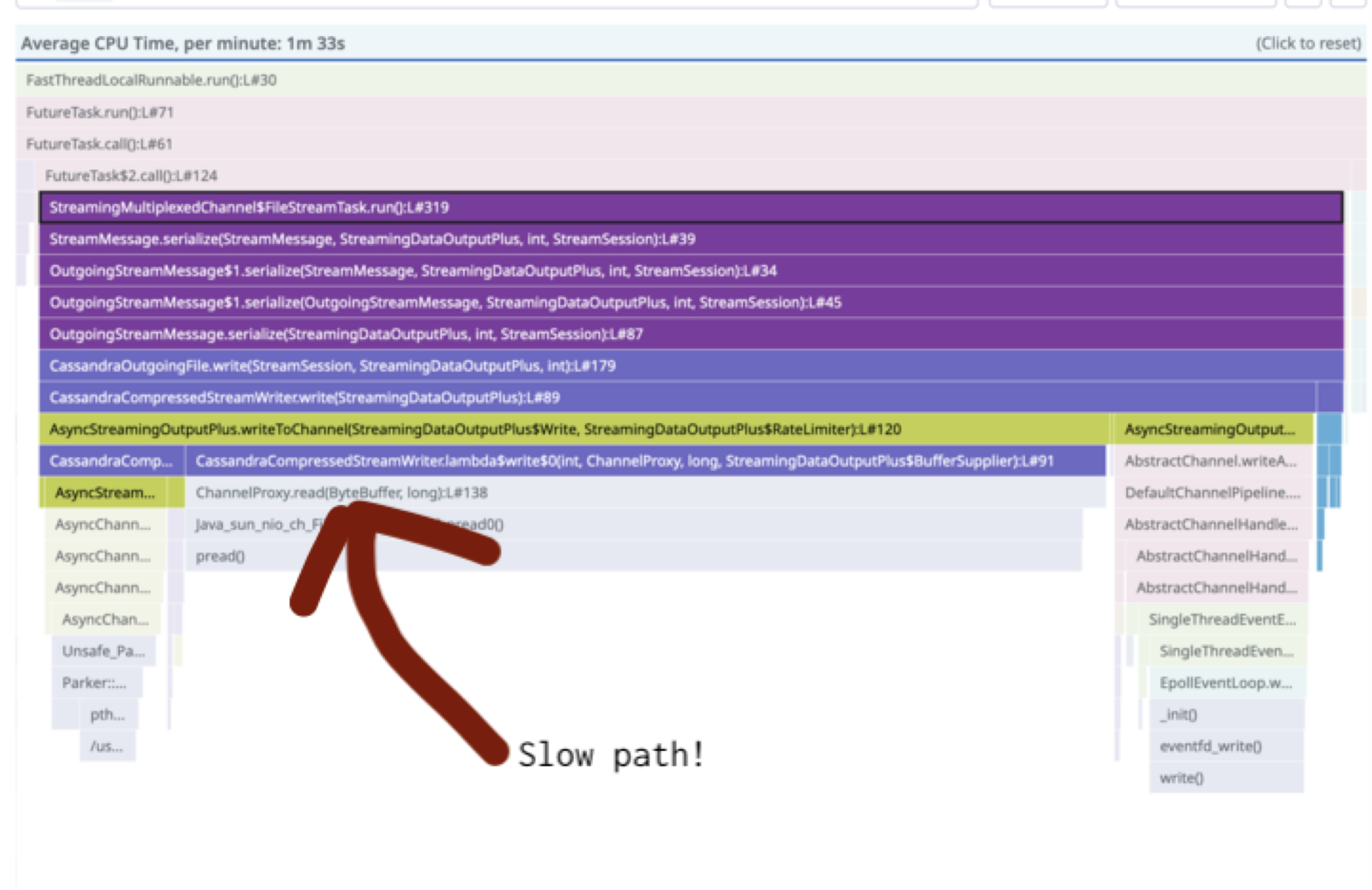
The Slow Fallback Path

If either of the two above options can’t be used, Cassandra will fall back on the slow path. This consists of:

• Identifying all the relevant chunks that need to be streamed
• Reading in 64KB of data at a time into a buffer
• “Fusing” segments together
• Sending over the network

This is typically done from CassandraCompressedStreamWriter, although if you’ve disabled compression Cassandra will use CassandraStreamWriter.

How slow is the slow path? Well… it’s not great. I recently worked on a production environment where we saw it top out at 12MB/s. After some analysis, I noted what appears to be fairly straightforward optimizations that could be done to significantly improve the slow path, but as of now it remains unresolved.

Here’s a flame graph visualization showing where the time is spent in one test:

Optimizations

As I mentioned earlier, the fast paths can only be used when the entire SSTable is going to be streamed. What does this even mean? Well, the data in an SSTable is sorted by token order. The first partition in the data file has the smallest token value, and the last partition has the highest value.

We can inspect the metadata with the sstablemetadata command to find out what these values are (output truncated for readability):

$ tools/bin/sstablemetadata path/to/some-Data.db
...
First token: -9156174751224047095 (001.0.900787)
Last token: 9054389320516065254 (001.0.43123)
...

If the node that’s joining the cluster owns the entire token range that this SSTable contains, then this SSTable is eligible to be streamed on one of the fast paths.

If there is another node that owns a token in the middle of this range, then bad news, the SSTable will be sent over the slow path. We don’t want send the entire SSTable because we’d be sending data the destination node won’t own. We could end up transferring several TB worth of data every time we expand the cluster, which works against our goal of minimizing streaming time, and can overload the destination node’s storage capacity.

You can see all the tokens owned by each node using the nodetool ring command (output truncated):

$ nodetool ring

Datacenter: datacenter1
==========
Address         Rack        Status State   Load            Owns                Token
                                                                               9072795746529349862
127.0.0.1       rack1       Up     Normal  669.86 KiB      100.00%             -8130428321499609781
127.0.0.1       rack1       Up     Normal  669.86 KiB      100.00%             -7163064078421074282
127.0.0.1       rack1       Up     Normal  669.86 KiB      100.00%             -5573059525907175644
...

Now that we know when the optimization kicks in, how can we ensure it does? There’s two things we can do.

Limit Usage of Virtual Nodes

Virtual Nodes (vnodes) were introduced in Cassandra 1.2and were enabled by default in 2.0. The setting to enable them at the time was:

num_tokens: 256

Unfortunately, using them didn’t really solve the performance and scalability problems they were meant to solve, and in a lot of cases made both worse. Sometimes way worse. Joey Lynch and Josh Snyder of Netflix published a paper, Cassandra Availability with Virtual Nodes, showing how increased numbers of vnodes lead to a decreased availability. They also increase the time it takes to run repair, query secondary indexes, scan tables, and unfortunately, they make it much less likely that you’ll be able to take advantage of the fast streaming path. In fact, they make it incredibly unlikely. I’ve worked with a few larger clusters running 256 vnodes per node and they were incredibly unstable.

Why Does This Impact Streaming?

When a new node joins a cluster, it picks it’s own tokens (shorthand for virtual nodes). This was random with the initial implementation. In modern Cassandra, they’re distributed around in the ring in a manner that should be roughly balanced.

The more tokens a node generates, the more likely it is to generate a token that lands in the middle of an existing SSTable. Once that happens, that SSTable can’t be streamed in its entirety to the new node, and the data is sent over the slow path.

Because of all the issues that high virtual node counts introduced, the default was lowered to 16 and some optimizations were done to improve their distribution. Despite the change, I recommend using no more than 4 nodes. There are benefits when used at this level, mainly that you can incrementally expand a cluster. There is no situation where I would recommend more.

The following should be set in your cassandra.yaml to use 4 virtual nodes:

num_tokens: 4

Important!: If you’re looking to change the number of virtual nodes in your cluster, the safest way is to create a new datacenter, and make the change there. There’s not a great way of doing it within a DC, and it can’t be done on a node that’s already joined in the cluster. Going into more detail would be a topic for a future post.

Limit SSTable Size Using Compaction Strategy

The default compaction strategy has been SizeTieredCompactionStrategy (STCS) for years. There are countless problems with it, one of which being that it generates larger and larger SSTables. Larger SSTables means larger token ranges in a data file, which means we’re more and more likely to have new nodes generate tokens that land in the middle of those SSTables. When that happens, we hit the slow path. Unfortunately, the same issue affects TimeWindowCompactionStrategy, which is used in many large time series clusters. At the time I recorded this video, for a lot of time series use cases there was no alternative option. Fortunately with Cassandra 5, that’s changed.

At a high level, what we need is a compaction strategy that limits SSTable size. We’ve had LeveledCompactionStrategy (LCS) available for years, but with Cassandra 5, we gained UnifiedCompactionStrategy (UCS).

I’ve spent a bit of time digging into the concepts behind UCS, and I can say that both conceptually, and practically, UCS is a brilliant body of work. It can be configured to replace all other compaction strategies. If there’s interest, in a future post I’ll dive deeper into the gory details of how UCS works and its configuration options, but for now, I’ll stick to the basics.

If you’re currently using STCS with default options, you can switch to UCS by doing the following:

ALTER TABLE mykeyspace.foo 
    WITH COMPACTION = 
        {'class': 'UnifiedCompactionStrategy', 
         'scaling_parameters': 'T4'};

UCS can also replace LCS:

ALTER TABLE mykeyspace.foo 
    WITH COMPACTION = 
        {'class': 'UnifiedCompactionStrategy', 
         'scaling_parameters': 'L10'};

To replace TWCS, you should follow the advice in my Time Series video, but use UCS instead of TWCS. If you’ve already been using multiple tables, you can incrementally convert the other tables to use UCS.

If you haven’t upgraded to Cassandra 5 yet, only tables using LCS can take advantage of the fast path. The biggest tables are probably going to be more write heavy, making them more likely to use STCS or TWCS in the past. Even if there were no additional benefits to 5.0, upgrading would be worth it for UCS by itself.

Once you’re using UCS, compaction has caught up, and you’re not using a lot of vnodes, most of your SSTables will be eligible for the two fast paths.

Conclusion

Optimizing Apache Cassandra for cost efficiency is a multi-faceted challenge, and streaming performance plays a crucial role in this equation. By understanding and implementing the optimizations outlined in this post, you can significantly increase your node density and reduce operational costs:

1. Enable Zero Copy Streaming by setting stream_entire_sstables: true in your cassandra.yaml configuration to take advantage of the most efficient streaming paths when possible.
2. Limit virtual nodes to 4 or fewer to maximize the chances of using the fast streaming path while still maintaining good token distribution.
3. Use the right compaction strategy - UnifiedCompactionStrategy in Cassandra 5.0 provides exceptional control over SSTable sizes, helping to ensure more SSTables can be streamed in their entirety.

These optimizations together lead to better streaming efficiency, which leads to faster node replacements and scaling operations, which enables higher node density, which in turn reduces your total node count and operational costs. As our example demonstrated, this approach can save your organization huge sums of cash while simultaneously improving cluster resilience.

The ability to efficiently handle more data per node isn’t just a technical nicety, it’s a significant business advantage. When you can double your storage capacity by simply expanding your volumes rather than doubling your node count, you’re making a strategic choice that impacts both your bottom line and your operational complexity.

In upcoming posts, I’ll explore additional Cassandra optimizations that can help you further reduce costs by increasing node density.

Remember, these optimizations are most effective on Cassandra 5.0 or later, which includes significant improvements specifically designed for higher node density operations. If you’re still running older versions, upgrading should be a priority on your roadmap!