Optimizing Cassandra Repair for Higher Node Density

• Wed, Oct 22, 2025
• 12-minute read

This is the fourth post in my series on improving the cost efficiency of Apache Cassandra through increased node density. In the last post, we explored compaction strategies, specifically the new UnifiedCompactionStrategy (UCS) which appeared in Cassandra 5.

• Streaming Throughput
• Compaction Throughput and Strategies
• Repair (you are here)
• Query Throughput
• Garbage Collection and Memory Management
• Efficient Disk Access
• Compression Performance and Ratio
• Linearly Scaling Subsystems with CPU Core Count and Memory

Now, we’ll tackle another aspect of Cassandra operations that directly impacts how much data you can efficiently store per node: repair. Having worked with repairs across hundreds of clusters since 2012, I’ve developed strong opinions on what works and what doesn’t when you’re pushing the limits of node density.

As with other topics in this series, repair performance is deeply intertwined with seemingly unrelated configuration choices. To add to the confusion, like many other aspects of complex distributed systems, these relationships aren’t always additive. In the case of incremental repair and compaction strategy choice, they can be multiplicative and sometimes antagonistic. For example, enabling incremental repair with SizeTieredCompactionStrategy (STCS) can result in dramatically worse performance than simply running subrange repair.

The optimization I discuss in these posts often be implemented together to achieve the dramatic improvements needed for high-density deployments. This post will explain why these subsystems are interconnected, and help you understand their behavior so you can configure them properly. I will avoid using specific numbers here as I’ve found the correct settings can vary between environments, and instead focus on the core concepts so you can apply it to your own clusters.

A Repair Primer

Repair is Cassandra’s process for ensuring data consistency across replicas. When a node goes down or experiences network partition, it may miss writes. Repair identifies and resolves these inconsistencies by comparing data across replicas and synchronizing any differences. Without regular repair, these inconsistencies can accumulate over time, leading to data loss when nodes are permanently removed from the cluster or when consistency levels don’t require reading from all replicas.

You can also find your deleted data gets resurrected, if a tombstone is garbage collected before it can be fully replicated.

There are two mechanisms Cassandra provides for repairing your entire dataset (excluding read-repair). Both are based on Merkle trees, although they’re used slightly differently and have different characteristics with regard to both performance and reliability.

Merkle trees are hierarchical hash structures that allow efficient comparison of large datasets. By hashing small chunks of data and then hashing those hashes together into a tree structure, you can quickly identify which specific portions differ between replicas without exchanging and comparing every byte. Without something like this it would be impactical to try to proactively resolve data inconsistencies.

Repair Orchestration: Don’t Do It Manually

Before I get into the weeds of this post, let’s address an important decision: never run repairs manually with cron scripts or ad-hoc nodetool commands.

I have seen too many instances where people have use cron with custom scripts to manage repair. It rarely goes well.

Managing repair manually becomes impractical at any scale, especially with high-density nodes. Manual repair scripts inevitably fail to handle:

• Token range calculation and segmentation
• Failure detection and automatic retries
• Coordination across multiple nodes
• Anti-compaction overhead tracking
• Progress monitoring and alerting
• Load-aware scheduling

You need a orchestration layer that can handle all of the nuance of repair. In the world of open source, I recommend Reaper. AxonOps has a very nice commercial adaptive Repair service that’s a bit more sophisticated. Hosted solutions like Instaclustr and Astra manage this for you.

Let’s move on and take a look at our repair options.

Full Repair

This is the most basic repair approach that repairs all data in the entire dataset.

While comprehensive and conceptually simple, full repair becomes a significant operational burden as data volumes grow. On a 10TB node, full repair will read and hash several terabytes of data to build merkle trees, consuming hours of I/O bandwidth and CPU time. The cost scales linearly with data volume. Doubling the data per node roughly doubles the repair time and resource consumption. This linear scaling becomes problematic in high-density deployments where nodes might hold 20TB or more. The time spent repairing also becomes less and less efficient over time, since repairing data that was already repaired doesn’t generally provide much value.

Incremental Repair

Introduced in Cassandra 2.1 to address the above inefficiency of full repair by tracking which SSTables have already been repaired. Rather than repairing data repeatedly, we repair it once, then mark it as repaired. In the next repair session, we only repair the unrepaired data.

It makes a lot of sense - why would you need to keep repairing data over and over? You want to repair your new data as quickly as possible, and repairing a multi-pb dataset in a few hours just isn’t practical.

The mechanism works by looking at all the SSTables are that going to be part of this repair, and first splitting any SSTables that have some data that will be repaired from data that won’t be. This is called anti-compaction. It’s an important step, because after the data is successfully repaired, it marks the SSTables as “repaired”. This is an update to the metadata only, so it’s important that all the data in the SSTable was actually repaired. We need to ensure that we transactionally move the data into a repaired state. If we don’t do this right, we can end up running into some serious issues later on. For detailed explanation, see Alex Dejanovski’s excellent blog post on incremental repairs.

Subsequent repairs only need to validate unrepaired SSTables that have been modified through compaction. This approach dramatically reduces the amount of data that needs to be read and compared on each repair cycle.

Here’s why incremental repair matters for high-density nodes. Let’s use 10TB / node as an example:

Reduced I/O Load: Instead of reading 10TB of data to build merkle trees, running incremental repair hourly might only to read a few GB of new data written since the last repair. This several orders of magnitude reduction in I/O directly translates to faster repair completion and less interference with application workloads. The I/O saved is particularly valuable on high-density nodes where disk bandwidth is already under pressure from application reads, writes, and compaction. Remember, reducing density doesn’t decrease overall cluster query throughput, so as you remove nodes from the cluster, each node needs to manage a higher RPS.

Predictable Resource Usage: With full repair, resource consumption is proportional to total data volume. A node with 20TB requires about twice the IO and CPU overhead of a 10TB node to build a merkle tree. Incremental repair shifts this dynamic: resource usage becomes proportional to the rate of new writes, which is typically far more stable than total data volume. This predictability makes capacity planning much more straightforward and allows you to run repairs more frequently without fear of overwhelming node resources.

Faster Completion Windows: In high-density environments where you might have 20TB+ per node, completing a full repair within a reasonable window becomes challenging. I’ve seen repairs take months on dense nodes that haven’t been optimally configured. Incremental repair, when run frequently, can complete in under an hour because it only processes the delta since the last successful repair. This faster completion enables more frequent repair cycles, which in turn keeps the amount of unrepaired data small and makes each subsequent repair even faster.

Better Scaling Characteristics: As you increase node density, the gap between full and incremental repair is massively amplified. For example, going from 5TB to 20TB per node might increase full repair time from a week to a month, but incremental repair time might only increase from 10 minutes to about half an hour.

Incremental repair is not without complexity. Cassandra needs to split SSTables that span repair boundaries through anti-compaction. This rewriting of data can itself be expensive, particularly with STCS. Adding to the challenge is that simply enabling incremental repair without addressing the compaction strategy can actually make things worse. I recently worked on a cluster where Reaper estimated it would take around a year to repair due to all the anti-compaction.

Important note:

Clusters Running Versions < 4.0: Incremental repair in Cassandra 2.x and 3.x had significant implementation issues that made it unreliable for production use:

• State tracking failures: Repaired/unrepaired state could occasinally become inconsistent across replicas
• SSTable proliferation: This resulted in the sudden accumulation of thousands of small SSTables, degrading read performance, and creating a massive compaction backlog, sometimes resulting in outages.

In practice, data could remain out-of-sync even after “successful” repairs, leading most operators to avoid incremental repair entirely. .

The 4.0+ Solution: Cassandra 4.0 fundamentally rewrote incremental repair with improved state tracking, reliable anti-compaction, and better compaction integration. The new implementation addresses all the core problems from earlier versions, making incremental repair production-ready and the recommended default for 4.0+ clusters.

SubRange Repair

SubRange repair is a powerful technique for managing repair on high-density nodes by dividing the token range into smaller, more manageable segments. Instead of repairing an entire node’s token range at once, subrange repair allows you to repair specific token ranges, giving you fine-grained control over the repair process. This was a standard practice long before people were running dense nodes, and is the reason why we adopted Reaper when I was at The Last Pickle.

SubRange repair operates by:

1. Dividing the token space: The node’s token range is split into smaller segments
2. Repairing incrementally: Each segment is repaired independently, reducing memory overhead
3. Parallelizing carefully: Multiple small repairs can run with controlled parallelism
4. Reducing impact: Smaller repairs mean less impact on ongoing operations

Benefits of SubRange Repair:

1. Memory efficiency: Each repair session uses less memory for Merkle trees
2. Predictable duration: Smaller segments complete in predictable time windows
3. Failure isolation: If a repair fails, only a small segment needs to be retried
4. Scheduling flexibility: Repairs can be spread across maintenance windows
5. Reduced streaming: Less data transferred if inconsistencies are localized

However, while repair is essential for cluster health, it’s also one of the most resource-intensive operations in Cassandra. As node density increases, the challenges become more pronounced:

1. Resource Consumption: Even subrange repair uses significant CPU, memory, and disk I/O
2. Coordination overhead: Managing multiple subrange repairs requires orchestration
3. Token calculation complexity: Manual token calculations are error-prone
4. Progress tracking: Monitoring which segments have been repaired requires tooling

The challenge is clear: how do we maintain data consistency through regular repairs while minimizing the performance impact on high-density nodes? The answer is proper orchestration tooling, not manual scripts.

Optimizing Repair for High Density Nodes

Here are the key strategies for optimizing repair in high-density environments:

Use Incremental Repair (Cassandra 4.0+ Only)

If you’re on Cassandra 4.0 or later, incremental repair has been significantly improved and I highly recommend it. It’s now the default repair method and provides the best balance of efficiency and reliability.

If you have a large dataset and you want to migrate to incremental repair,

For versions prior to 4.0, incremental repair had significant issues and should be avoided. Use subrange repair exclusively instead.

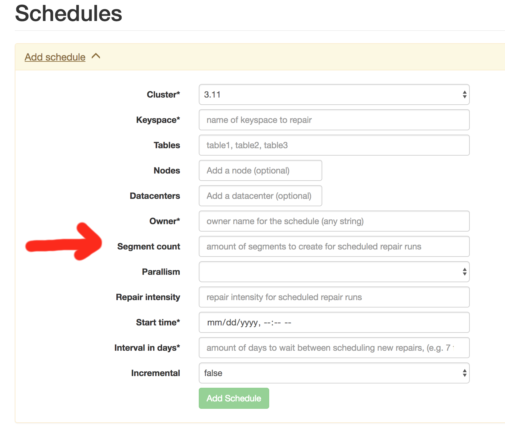
Tune Segment Size

With high node density and fewer nodes, each token range becomes larger. When setting up a repair schedule with Reaper, you’ll see a segment count field. I can’t understate how important it is to evaluate this setting in conjunction with picking an appropriate compaction strategy.

Here’s where things get rough - tables using SizeTieredCompactionStrategy can cause repair time to balloon by several orders of magnitude. This is because STCS can generate pretty massive SSTables, and anti-compaction needs to split them apart. With really small ranges, you could end up splitting a multi-hundred GB SSTable several times. Your nodes can find themselves rewriting the same data so many times that they never actually get to do any actual repair work, they’re just rewriting data.

Using fewer segments means you’ll repair more data at once, but with STCS you’ll still run the risk of needing to repair fairly large SSTables. We can do better.

Addressing the STCS Problem:

For Cassandra 5.0+, the best solution is to migrate to UnifiedCompactionStrategy (UCS), which I recommend for 100% of workloads. UCS handles incremental repair’s anti-compaction requirements much more efficiently than STCS. For a detailed discussion of UCS and migration strategies, see my previous post on compaction strategies.

For versions before 5.0, consider using LeveledCompactionStrategy (LCS) if your workload can keep up with its compaction requirements. LCS maintains smaller, fixed-size SSTables that work well with anti-compaction.

Use Fewer vNodes

As mentioned in the first post about streaming, the number of virtual nodes (vNodes) per physical node significantly impacts repair performance.

You can’t change the number of tokens on a running node, and you shouldn’t try to do the dance where you add nodes to a DC then remove them. You’ll end up with a node that is a replica for every other node in the cluster. To address this properly, you’ll need to add a new datacenter with the new num_tokens setting.

The Future of Repair: Autonomous Operations

The repair optimizations discussed in this post represent the current state of production systems, but Cassandra’s repair mechanisms are evolving rapidly. Two major developments will fundamentally change how we think about repair in high-density deployments.

Automatic Repair in Cassandra 6.0

Cassandra 6.0 introduces automatic repair capabilities as part of CEP-37 that remove much of the operational burden from maintaining data consistency. This feature represents a significant leap forward in making Cassandra more autonomous and operator-friendly.

I will discuss this more in a future post.

Mutation Tracking: The End of Traditional Repair

An even more transformative change will be CEP-45: Mutation Tracking, which fundamentally reimagines how Cassandra maintains consistency across replicas.

Traditional repair, even with all optimizations, still requires:

1. Reading data from disk to build Merkle trees
2. Comparing trees between replicas
3. Streaming mismatched data
4. Anti-compacting SSTables (for incremental repair)

Mutation tracking eliminates most of these steps by:

• Assigning globally unique IDs to every write operation
• Maintaining compact summaries of which mutations each replica has received
• Comparing mutation IDs instead of actual data
• Streaming only missing mutations rather than entire partitions

I’ll have a dedicated post on this topic in the future as well.

Conclusion

Efficient repair processes are essential for maintaining data consistency in high-density Cassandra deployments. By implementing the strategies outlined in this post, you can significantly reduce the performance impact of repairs while ensuring data remains consistent across your cluster.

Remember, these optimizations are most effective on Cassandra 4.0 or later, where incremental repair has been significantly improved. If you’re still running older versions, upgrading should be a priority on your roadmap. I strongly recommend upgrading all the way to Cassandra 5.0, as the cost of running clusters has significantly decreased due to the improvements in node density.

In our next post, we’ll explore how efficiency improvements in query throughput can help improve node density.

If you found this post helpful, please consider sharing to your network. I'm also available to help you be successful with your distributed systems! Please reach out if you're interested in working with me, and I'll be happy to schedule a free one-hour consultation.